Economic Causality

Finding out what affects what in the markets

Jul 18, 2026

For a while I have been running some forecasting models that handle macros, indexes and prices for futures/crypto/forex and stocks in order to see if I could produce something that could predict the markets distribution with any kind of accuracy.

The Model Architecture

These models take the form of Gradient Boosted Trees (GBTs) that are binary classifiers over a specific part of the normal distribution with a running standard deviation normalisation. Lots of tricks are employed in terms of the feature selection, calibration and further normalisation of these features but I will save that for another post, right now I just want to talk about what these models can tell us about how the financial world interacts.

These models when run together form a panel that can walk itself forward, and with vine copulas tying the joint distributions of these tickers together you end up with walks like the following:

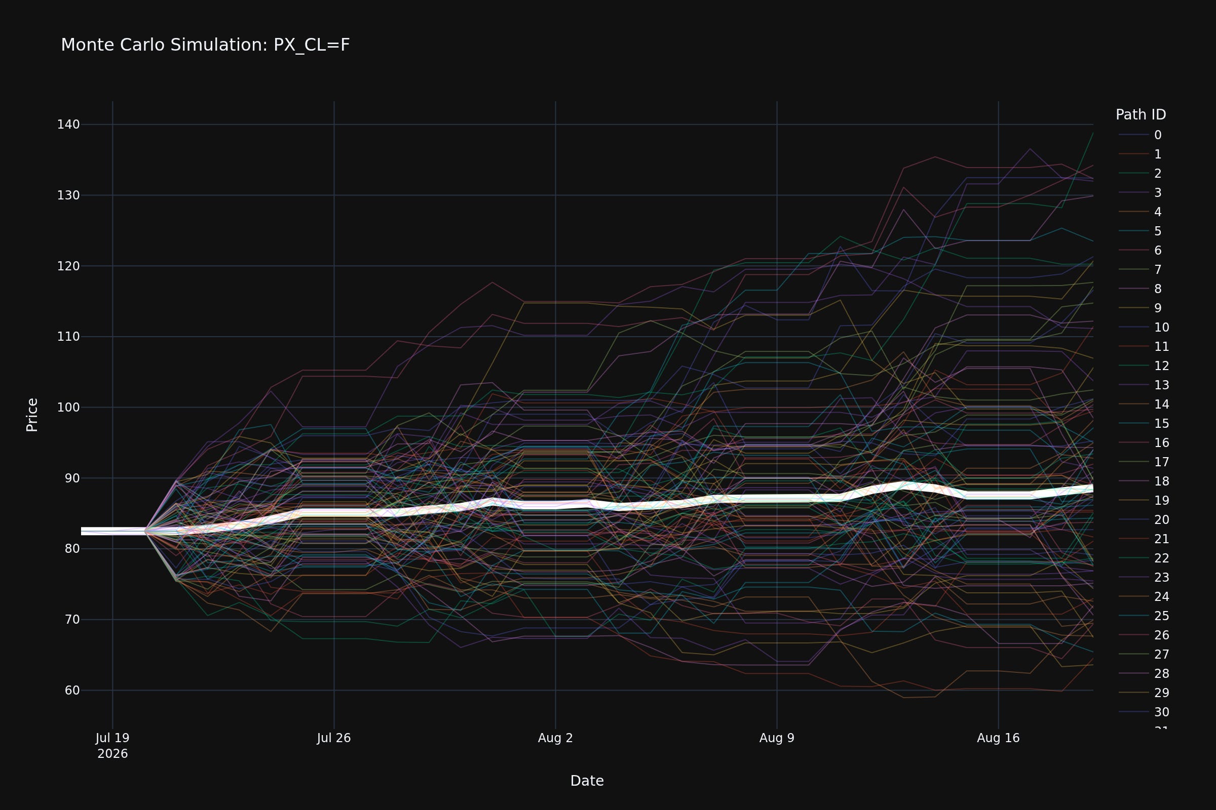
What this is showing us, is that if you walk this panel forward 32 days, and do that 100 times randomly selecting different parts of the cumulative distribution function, you end up with a distribution, and in this case you will notice that on crude oil futures, the distribution skews up much more than it skews down, and this is reflected in the median line moving up towards $90 from a starting point of about $82.

Panel Causality

Now the interesting thing here, is each of these models can use generated features from any of the members of the panel, and the panel currently has the following members:

- MACRO_^IRX : 13 WEEK TREASURY BILL
- MACRO_BAMLH0A0HYM2 : ICE BofA US High Yield Index Option-Adjusted Spread
- MACRO_CPIAUCSL : Consumer Price Index for All Urban Consumers: All Items in U.S. City Average
- MACRO_DCOILWTICO : Crude Oil Prices: West Texas Intermediate (WTI) - Cushing, Oklahoma
- MACRO_DGS10 : Market Yield on U.S. Treasury Securities at 10-Year Constant Maturity, Quoted on an Investment Basis
- MACRO_DTWEXBGS : Nominal Broad U.S. Dollar Index
- MACRO_FEDFUNDS : Federal Funds Effective Rate
- MACRO_GDP : Gross Domestic Product
- MACRO_INDPRO : Industrial Production: Total Index
- MACRO_M2SL : M2
- MACRO_T10Y2Y : 10-Year Treasury Constant Maturity Minus 2-Year Treasury Constant Maturity
- MACRO_T10YIE : 10-Year Breakeven Inflation Rate
- MACRO_TRFVOLUSM227NFWA : Vehicle Miles Traveled
- MACRO_UNRATE : Unemployment Rate
- MACRO_VIXCLS : CBOE Volatility Index: VIX
- PX_BITO : ProShares Bitcoin ETF
- PX_BTC-USD : Bitcoin USD Price
- PX_CL=F : Crude Oil
- PX_EEM : iShares MSCI Emerging Markets ETF
- PX_ETH-USD : Ethereum USD Price
- PX_EURUSD=X : EUR/USD
- PX_GC=F : Gold
- PX_HG=F : Copper
- PX_HYG : iShares iBoxx $ High Yield Corporate Bond ETF
- PX_IWM : iShares Russell 2000 ETF
- PX_QQQ : Invesco QQQ Trust
- PX_SI=F : Silver
- PX_SMH : VanEck Semiconductor ETF
- PX_SPY : SPDR S&P 500 ETF
- PX_SPYD : State Street SPDR Portfolio S&P 500 High Dividend ETF
- PX_TLT : iShares 20+ Year Treasury Bond ETF
- PX_USDJPY=X : USD/JPY
- PX_VNQ : Vanguard Real Estate Index Fund ETF

So because each of these models can see features from all the other tickers, we eventually end up with a models that assign certain importance’s to these features, which means we can see exactly how much these different tickers / macros influence each other, thus causing change. It’s very important to note that this is significantly different to a correlation map, or a PCA reduction map, this is indicating that the models are directly using this data to come up with an optimal forecast and are assigning an importance to that. Mapping that into a 2D graph yields the following result:

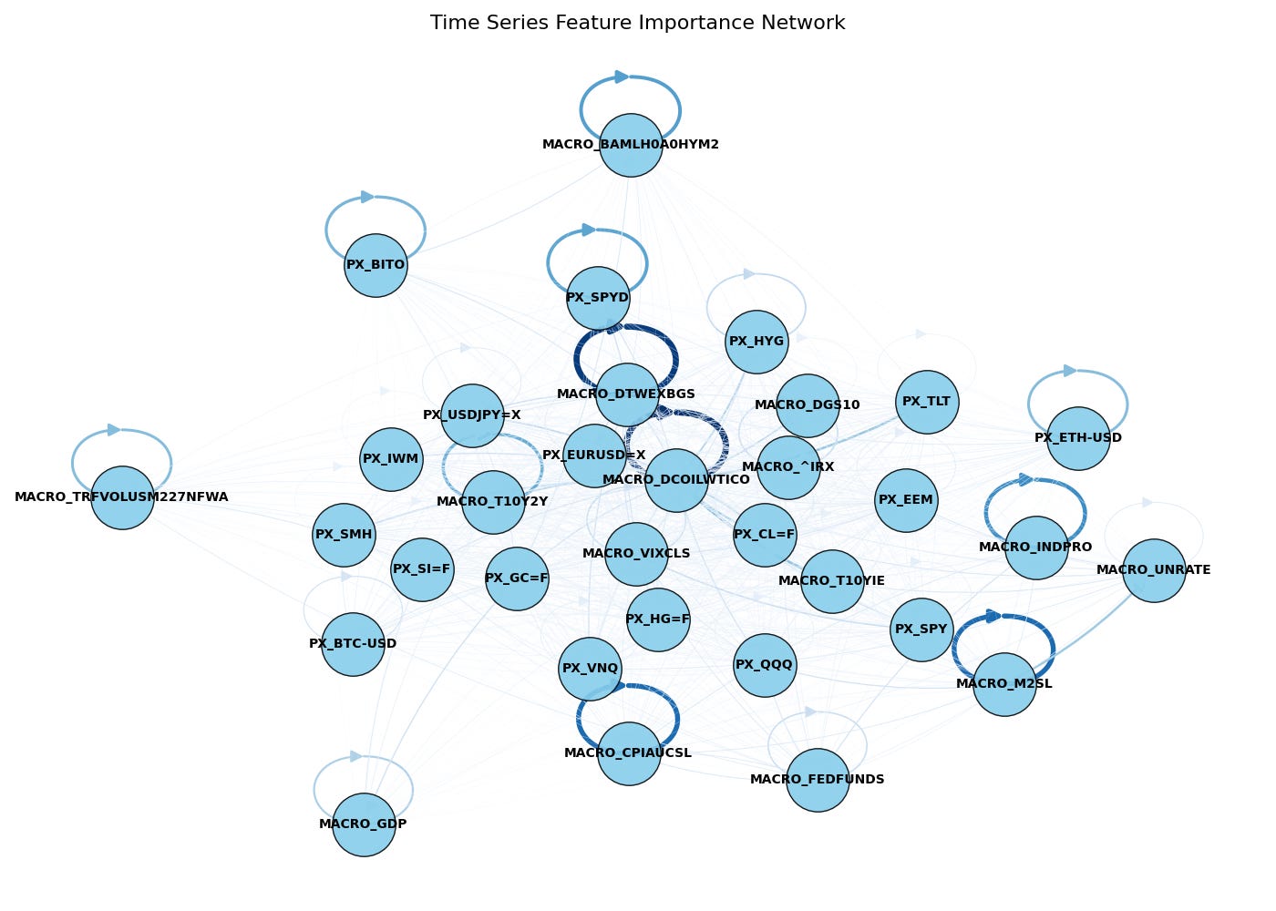
Now this is really fascinating to look at, because you can see via the “halos” these tickers produce that some of these tickers are self-referential. Now that doesn’t necessarily mean they are actually self-referential, it just means we haven’t found a good way to model these tickers that is significantly better than the information we get just from how these tickers have behaved in the past. Just glancing at the graph we have the following notable self-referential tickers:

ICE BofA US High Yield Index Option-Adjusted Spread
Nominal Broad US Dollar Index
Crude Oil Prices: West Texas Intermediate (WTI) - Cushing, Oklahoma
M2
Consumer Price Index for All Urban Consumers: All Items in U.S. City Average

Now this is quite important, because if we rank our nodes by causality (closer to the center), we get the following:

Crude Oil Prices: West Texas Intermediate (WTI) - Cushing, Oklahoma (35.3027)
Nominal Broad U.S. Dollar Index (22.0868)
CBOE Volatility Index: VIX (15.9238)
10-Year Treasury Constant Maturity Minus 2-Year Treasury Constant Maturity (14.8259)
Crude Oil (13.8168)

Its interesting that these tickers are driving so many of our predictions, yet our system struggles to predict them without self-referencing, showing that there are big improvements to be made just by finding data that can suggest what moves these tickers.

What if we rank our nodes by lowest causality (closer to the edge)? This results in the following:

Gross Domestic Product (4.7056)
ICE BofA US High Yield Index Option-Adjusted Spread (5.8670)
Federal Funds Effective Rate (6.2107)
Vehicle Miles Traveled (6.3316)
Unemployment Rate (6.4109)

Very interesting to see things like GDP or Unemployment Rate be so uncausal to the rest of our panel, this is probably due to these metrics being lagging indicators of other factors across the market.

LLM Reasoning

With this dataset can we get “quantamental” and start reasoning about some of these quantitative features using LLMs to analyse and maybe produce some insight that can be more approachable to humans rather than computers? Lets give it a go.

To do this, first lets feed in the top 5 feature importance’s of the model, the feature script that generated them, and its association with other tickers in the panel, and tell it to write some reasoned arguments as to what it thinks may be going on with the different feature importance’s and what is suggests about the relationship between the 2 nodes. This produces documents like the following:

# Target: MACRO_^IRX

## Top 5 Features:
- `MACRO_DCOILWTICO_kurt_5_lag1`: 0.2884
- `MACRO_DTWEXBGS_kurt_5_lag10`: 0.1499
- `PX_SPYD_beta_5_rmean60`: 0.1441
- `PX_SI=F_skew_200_rstd200`: 0.1073
- `PX_SMH_kurt_10_lag30`: 0.1062

---

## Quantitative Reasoning

### Executive Summary

The target asset, **`MACRO_^IRX`** (13-Week US Treasury Bill yield), represents the ultra-short end of the risk-free curve. Volatility breakouts (standard deviation breaches) in this asset are primarily driven by shifts in monetary policy expectations (Federal Reserve rate path), systemic liquidity shocks, and sudden changes in inflation expectations. 

The Gradient Boosted Trees (GBT) model has selected a highly logical, non-linear mix of features to predict these breakouts. Rather than relying on simple directional momentum, the model exploits **higher-order moments (kurtosis and skewness)** and **smoothed systematic risk metrics (beta)** across key macro proxies: energy (WTI), currencies (USD), yield-sensitive equities (SPYD), precious metals (Silver), and cyclical growth drivers (Semiconductors). 

---

### Regime Indicators

The GBT model utilizes long-lookback, smoothed indicators to establish the structural macro environment. These features act as the "state variables" that dictate whether the market is in a regime highly sensitive to short-term rate shocks.

*   **`PX_SPYD_beta_5_rmean60` (Importance: 0.1441) — Yield-Sensitive Equity Systematic Risk:**
    *   *Quantitative Rationale:* `SPYD` (S&P 500 High Dividend ETF) consists of high-yielding, bond-proxy equities (e.g., Utilities, Real Estate). The 5-period rolling beta measures the short-term sensitivity of these yield-sensitive stocks to the broader market, while the 60-period rolling mean smooths this metric to capture structural regimes. 
    *   *Market Dynamics:* A persistent shift in the beta of dividend-paying stocks indicates a regime change in how equities digest interest rate risk. When this smoothed beta is elevated or depressed, it signals to the GBT model whether the equity market is trading on growth or discount-rate dynamics, which directly precedes volatility regimes in short-term funding rates (`^IRX`).
*   **`PX_SI=F_skew_200_rstd200` (Importance: 0.1073) — Precious Metals Tail-Risk Instability:**
    *   *Quantitative Rationale:* This feature measures the 200-period rolling standard deviation of Silver’s 200-period return skewness. It represents the *volatility of tail-risk asymmetry* in a key monetary/industrial metal.
    *   *Market Dynamics:* Silver serves as a hybrid asset—highly sensitive to both industrial demand and monetary inflation hedging. High volatility in its long-term skewness indicates unstable market expectations regarding inflation and real yields. The GBT model exploits this instability as a leading indicator of structural regime shifts in inflation expectations, which ultimately force abrupt adjustments (volatility breakouts) in short-term Treasury yields.

---

### Lead-Lag Relationships

The model utilizes specific time lags to capture the transmission delay between global macroeconomic shocks and the repricing of short-term US interest rates.

*   **`MACRO_DTWEXBGS_kurt_5_lag10` (Importance: 0.1499) — Delayed Currency Liquidity Transmission:**
    *   *Quantitative Rationale:* This feature measures the 5-period rolling kurtosis (tail-risk/extreme moves) of the Broad Trade-Weighted US Dollar Index, lagged by 10 periods.
    *   *Market Dynamics:* Extreme, leptokurtic moves in the US Dollar index signify acute global dollar funding squeezes or sudden shifts in international capital flows. The 10-period lag represents the transmission window: a shock in the FX/global liquidity channels takes approximately two weeks to filter down to domestic money markets, subsequently triggering volatility breakouts in 3-month T-Bills as domestic liquidity conditions tighten or ease.
*   **`PX_SMH_kurt_10_lag30` (Importance: 0.1062) — Cyclical Growth Shock Lead-Time:**
    *   *Quantitative Rationale:* This captures the 10-period rolling kurtosis of the Semiconductor ETF (`SMH`), lagged by 30 periods (approximately 1.5 calendar months).
    *   *Market Dynamics:* Semiconductors are the ultimate leading indicator of global industrial production and risk-on sentiment. Extreme tail-events (high kurtosis) in `SMH` signal sudden demand shocks or supply-chain disruptions. The GBT model utilizes a 30-period lag because real-economy growth shocks take roughly 1 to 2 months to impact macroeconomic data releases, which subsequently force the Federal Reserve to adjust the policy rate path, causing a delayed volatility breakout in `^IRX`.

---

### Cross-Asset Dynamics

The most powerful predictor in the model captures immediate, non-linear shocks from the energy sector, which act as a direct proxy for cost-push inflation.

*   **`MACRO_DCOILWTICO_kurt_5_lag1` (Importance: 0.2884) — Immediate Energy-Driven Inflation Shocks:**
    *   *Quantitative Rationale:* This feature measures the 5-period rolling kurtosis of WTI Crude Oil spot prices, lagged by just 1 period. 
    *   *Market Dynamics:* Crude oil is the primary driver of short-term inflation expectations. A high 5-period kurtosis indicates sudden, extreme price spikes or crashes (fat-tailed behavior) rather than orderly trending behavior. Because the lag is only 1 period, the GBT model is exploiting an immediate cross-asset transmission channel: a sudden, violent shock in energy prices instantly alters the market's assessment of near-term inflation. This forces immediate repricing of the Fed's terminal rate, resulting in instant standard deviation breakouts in the 13-week T-Bill yield.

### Decision Tree Synthesis

The GBT model effectively constructs a multi-layered decision boundary:
1.  **State Identification:** It uses the smoothed systematic risk of bond proxies (`SPYD` beta) and the stability of inflation hedges (`SI=F` skewness volatility) to determine if the macro environment is fragile.
2.  **Macro/Liquidity Lags:** It monitors lagged shocks in global growth (`SMH` kurtosis at $t-30$) and global liquidity (`DTWEXBGS` kurtosis at $t-10$) to anticipate incoming rate adjustments.
3.  **Immediate Trigger:** It uses the immediate tail-risk of energy prices (`DCOILWTICO` kurtosis at $t-1$) as the tactical catalyst to trigger the binary prediction of a standard deviation breakout in `^IRX`.

Now we have these for each of the assets, there were obvious duplication’s (such as the kurtosis of WTI Crude Oil Prices), so now lets do some pruning, let’s ask an LLM to take all these reports, and distill what it considers to be the 5 most important drivers in the market, the following is the result of that (LLMs words):

Macro-Causal Insights: Panel Volatility Meta-Analysis

1. The Energy-Driven Jump-Diffusion Transmission Channel (Oil Kurtosis as a Term Premium Catalyst)

The overwhelming dominance of West Texas Intermediate (WTI) Crude Oil kurtosis features—specifically the ultra-short-term tactical indicator (kurt_5_lag1) and the medium-term structural indicator (kurt_10_lag30)—across virtually all asset classes (including sovereign yields, equities, high-yield credit, and precious metals) points to a universal causal mechanism: the non-linear transmission of energy-market tail risk into the global discount rate.

Mathematically, asset prices are modeled as continuous-time jump-diffusion processes:

$dS_t = \mu S_t dt + \sigma S_t dW_t + J_t S_t dN_t$

where dWt is a standard Brownian motion, dNt is a Poisson process with intensity λ, and Jt is the jump size distribution. Standard volatility models (e.g., GARCH) focus on the continuous diffusion component (σStdWt). However, the GBT model’s heavy reliance on kurtosis (the fourth standardized moment, κ=E[(X−μ)4]/σ4) indicates that volatility breakouts are fundamentally caused by the jump component (JtdNt).

When WTI Crude Oil exhibits high rolling kurtosis, it signals that the energy market has transitioned from a Gaussian diffusion regime to a jump-diffusion regime characterized by discontinuous price gaps. Because energy is a primary, non-substitutable input cost for global production, transport, and supply chains, a sudden, extreme energy price jump instantly destabilizes the inflation expectation component (πt(n)) of the nominal interest rate:

$y_t^{(n)} = \frac{1}{n}\sum_{i=0}^{n-1} \mathbb{E}_t[r_{t+i}] + \pi_t^{(n)} + \theta_t^{(n)}$

This sudden instability in πt(n) triggers a non-linear spike in the term premium (θt(n)) due to Knightian uncertainty. Fixed-income market makers, unable to price the long-end of the curve, immediately withdraw liquidity, causing standard deviation breakouts in long-duration Treasuries (PX_TLT, MACRO_DGS10). This fixed-income volatility instantly propagates to equities (PX_SPY, PX_QQQ) and credit (PX_HYG) via the discount rate channel, as the present value of future cash flows is violently recalculated.

2. Global Dollar Funding Squeezes and the Non-Linearity of Balance Sheet Constraints

The Trade-Weighted U.S. Dollar Index (MACRO_DTWEXBGS) serves as the ultimate barometer of global dollar funding liquidity. The GBT model’s reliance on USD tail-risk metrics (kurt_5_lag10) and trend efficiency (er_5_lag20) to predict volatility breakouts in emerging markets (PX_EEM), real estate (PX_VNQ), and foreign exchange (PX_USDJPY=X) is rooted in the causal mechanics of leveraged balance sheet constraints under Basel III regulations.

Global financial intermediaries (market makers and prime brokers) manage their risk-active balance sheets under strict Value-at-Risk (VaR) constraints:

$\text{VaR}_{\alpha} = \inf \{ L \in \mathbb{R} : \mathbb{P}(\text{Loss} > L) \le 1 - \alpha \}$

When the Trade-Weighted USD exhibits high trend efficiency (er_5) and sudden tail-risk (kurt_5), it indicates a rapid, directional appreciation of the dollar. Because the USD is the primary global funding currency, a rising dollar increases the value of dollar-denominated liabilities relative to local-currency assets on foreign bank balance sheets. This mismatch triggers a mechanical expansion in the intermediaries’ VaR.

To prevent regulatory capital breaches, these intermediaries must rapidly contract their balance sheets. They do this by:

Widening bid-ask spreads across all liquid instruments.
Demanding higher collateral haircuts.
Actively liquidating high-beta, non-dollar assets.

The 10-day lag (lag10) observed in the USD kurtosis features represents the operational latency of this margin-call and liquidation pipeline. It takes approximately two weeks for a global dollar funding squeeze to force international asset allocators to liquidate liquid proxies like Emerging Markets (PX_EEM) or Real Estate (PX_VNQ) to meet USD-denominated margin calls, resulting in a delayed but highly deterministic volatility breakout in those target assets.

3. Microstructural Phase Transitions and the Instability of Market Memory

A recurring precursor to volatility breakouts across the entire panel is the rolling standard deviation of autocorrelation and beta (e.g., MACRO_DCOILWTICO_autocorr_120_rstd5, PX_ETH-USD_beta_60_rstd60, MACRO_CPIAUCSL_er_10_rstd20). This statistical configuration represents a microstructural phase transition and the breakdown of market memory.

In a stable market regime, the serial correlation (autocorrelation) of returns is highly stable, reflecting a continuous, predictable flow of information and order execution. Mathematically, the market is in an equilibrium state where the feedback loop between trend-following (momentum) and mean-reverting (value) traders is balanced.

When the rolling standard deviation of autocorrelation (autocorr_rstdautocorr_rstd) or systematic risk sensitivity (beta_rstdbeta_rstd) spikes over an ultra-short window (e.g., rstd5), it indicates that the return-generating process is undergoing a structural bifurcation:

$\rho_{\tau, t} = \frac{\text{Cov}(R_t, R_{t-\tau})}{\text{Var}(R_t)}$

A rapid fluctuation in ρτ,t signals that the market is transitioning between a highly persistent, trending state (ρ→1) and a highly mean-reverting, congested state (ρ→−1).

During this transition, algorithmic execution models (such as CTA trend-followers and risk-parity funds) experience conflicting signals. As these models rapidly switch their positioning or deleverage to avoid whipsaws, they create massive imbalances in the limit order book. Market makers, observing the rapid instability of systematic risk (beta) and trend efficiency (er), face heightened adverse selection risk. To protect themselves, they pull liquidity from the order book. The sudden collapse in market depth (liquidity density) allows even modest order flows to cause massive, discontinuous price jumps, triggering a standard deviation breakout.

4. The Multi-Scale Temporal Cascade of Macroeconomic Shock Propagation

The GBT model’s feature profiles reveal a highly structured, multi-scale temporal cascade of lags (lag1, lag5, lag10, lag30) that maps the physical and financial transmission of macroeconomic shocks. This structured delay is not a statistical artifact; it is causally dictated by the operational horizons of different market participants and physical supply chains.

[T-30] Physical Supply Chain & Macro Reporting Lag (WTI Kurtosis Lag 30)
       │
       ▼
[T-10] Institutional Portfolio Rebalancing & FX Hedging Lag (USD Kurtosis Lag 10)
       │
       ▼
[T-5]  Systematic Strategy Deleveraging & CTA Rebalancing Lag (Oil/USD Kurtosis Lag 5)
       │
       ▼
[T-1]  Tactical Algorithmic Flow & Market Maker Gamma Hedging (Oil Kurtosis Lag 1)
       │
       ▼
[T-0]  VOLATILITY BREAKOUT IN TARGET ASSET

The Tactical Horizon (lag1): This represents immediate, flow-driven transmission. High-frequency trading algorithms, market-maker delta/gamma hedging profiles, and discretionary macro desks react within milliseconds to 24 hours of an extreme tail event (e.g., DCOILWTICO_kurt_5_lag1). This immediate flow triggers rapid repricing in highly liquid, financialized assets.
The Systematic Horizon (lag5 to lag10): This matches the weekly rebalancing schedules of systematic asset allocators, commodity trading advisors (CTAs), and risk-parity funds. When a shock persists or clusters over 5 to 10 days, it triggers portfolio risk-limit breaches, forcing systematic deleveraging and driving assets past their standard deviation thresholds.
The Macroeconomic/Physical Horizon (lag30): This corresponds to the physical reality of global trade and supply chains. An energy shock (kurt_10_lag30) takes approximately 30 to 45 days to physically propagate through manufacturing input costs, alter corporate profit margins, and manifest in official monthly macroeconomic data releases (such as CPI, PPI, and Industrial Production). The GBT model exploits this 30-day lag because it represents the exact window where physical economic deterioration forces central banks to adjust monetary policy, triggering secondary, structural volatility breakouts in interest-rate-sensitive assets.

5. Speculative Liquidity Sinks as Early-Warning Risk Thermometers

The highly consistent predictive power of speculative, high-beta assets—specifically Semiconductors (PX_SMH_er_10_rstd60) and Bitcoin (PX_BTC-USD_rsi_120_rstd10, PX_BITO_skew_5_rmean200)—over real-economy variables (such as Unemployment MACRO_UNRATE and High-Yield Credit MACRO_BAMLH0A0HYM2) is driven by the physics of global liquidity distribution.

Speculative assets with high financial leverage and 24/7 liquidity act as “liquidity sinks.” According to the global liquidity transmission theory, when central banks inject liquidity (M2M2) or when financial conditions loosen, capital does not flow immediately into physical capital expenditure or labor markets. Instead, it flows instantly into the most liquid, high-beta speculative instruments:

$\frac{d \text{Liquidity}}{dt} \to \text{Speculative Sinks (Crypto, Tech Options)} \to \text{Broad Equities} \to \text{Real Economy (CapEx, Jobs)}$

Conversely, when global liquidity begins to contract (due to quantitative tightening or rising discount rates), speculative capital is the first to flee. Because these assets are highly financialized and heavily traded via options and leveraged derivatives, they exhibit structural distribution shifts—such as rapid changes in trend efficiency (SMH_er_rstd) or momentum volatility (BTC_rsi_rstd)—long before the real economy registers the stress.

A sudden spike in the momentum volatility of Bitcoin or a breakdown in the trend efficiency of Semiconductors indicates that institutional “smart money” is quietly deleveraging and hoarding cash. This early liquidity withdrawal propagates outward from the speculative periphery to the core macro economy. By the time the credit markets (HYG) or labor markets (UNRATE) experience a volatility breakout, the speculative liquidity sinks have already exhibited highly anomalous, fat-tailed statistical configurations, making them highly sensitive, causal leading indicators of systemic risk-off events.

This analysis was very insightful, and relied entirely on the quantitative factors feeding it. I do firmly believe that the future of the financial industry lies in the space where these quantitative models and reasoning LLMs can operate to make something better than the sum of their parts.

Subsack

Discussion about this post

Ready for more?