
Wrangling Evals
Understanding the variance in evals helps us defeat it.

The more I speak to people in industries about how they are doing evals (evaluations of their agentic tasks), the more I believe there is a fundamental disconnect on how these processes work compared to normal deterministic programs. I have already written on some techniques you can use to reduce that variance in AIs favourite number, but reduction isn’t elimination, and you will still have to contend with scenarios where using the same input you may get answer A, or you may get answer B. This is of course very different to deterministic processes, like the kind you use when you build software, so naturally the industry is struggling to wrap its head around how to deal with this kind of process.
Luckily for us, although we have variance, there are ways to control this beast.
Law of Large Numbers and the Central Limit Theorem
In probability theory, the law of large numbers is a mathematical law which states that the average of the results obtained from a large number of independent random samples converges to the true value, if it exists.
So lets say, we are looking to figure out what the true accuracy is for our evaluations. To do this, we can just run our evaluations a large amount of times over a sample set representing our distribution, and over time the accuracy of our LLMs will converge to a single point. But how do we know when to stop?
In probability theory, the central limit theorem (CLT) states that, under appropriate conditions, the distribution of a normalized version of the sample mean converges to a standard normal distribution.
What the central limit theorem is telling us, is that while we are converging on our true accuracy, we are also converging on a normal distribution representing the LLMs accuracy. This is important, because it allows us to calculate our margin of error, and perform an early stop once we reach a good enough accuracy. For example if we want to be 95% confident in our accuracy, we can use a z-score of 1.96 (this corresponds to our 95% confidence) and multiply that by our standard error. To calculate the standard error for a binomial procedure (pass or fail) we can do the following:
So here we take our accuracy (p) from the previous process, the failure rate (the opposite of the accuracy), and the n (the number of runs). As you can imagine as the number of runs goes up, the larger the denominator gets, and the smaller our standard error becomes. Then finding our margin of error becomes a question of:
Lets put this into action via simulation, lets say we come up with a series of models, each with their own accuracy (and cost), and a series of tasks with some bias towards different models. By running them until we get a 95% confidence in our accuracy we come up with the following chart:
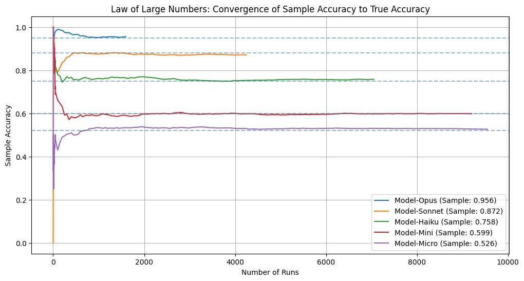
As you can see, our large of large numbers is performing exactly as expected! Here are the numeric results:
Model-Opus: Reached statistical significance after 1,615 runs.
  True Accuracy: 0.9500 | Final Sample Accuracy: 0.9560
  Final Margin of Error: 0.01000

Model-Sonnet: Reached statistical significance after 4,282 runs.
  True Accuracy: 0.8800 | Final Sample Accuracy: 0.8723
  Final Margin of Error: 0.01000

Model-Haiku: Reached statistical significance after 7,055 runs.
  True Accuracy: 0.7500 | Final Sample Accuracy: 0.7576
  Final Margin of Error: 0.01000

Model-Mini: Reached statistical significance after 9,228 runs.
  True Accuracy: 0.6000 | Final Sample Accuracy: 0.5989
  Final Margin of Error: 0.01000

Model-Micro: Reached statistical significance after 9,578 runs.
  True Accuracy: 0.5200 | Final Sample Accuracy: 0.5262
  Final Margin of Error: 0.01000
Our most accurate model converges the fastest and the least accurate the slowest, and it takes at least 1000~ runs for our best model and 10000~ for our worst model. Obviously this is too much to be of any use, the time and cost alone would be prohibitive. The good news, we only have to do this once, record our accuracy, and then we can exploit this known accuracy to do something much smarter.
Sequential Probability Ratio Test
Now that we know the accuracy of each of our models, we can use that information to subsequently perform much less runs to maintain our target confidence. To do this, we need to come up a system that runs an evaluation, and constantly determines whether it has enough information to stop.
First we need to calculate our lower and upper bounds, with our confidence interval of 95% we can define our alpha and beta as 0.05. To get our upper bound for the SPRT, we can use the following formula:
For our 95% confidence interval, this ends up being just shy of 3. Our lower bound is the same just inverted (-3).
Next we need to calculate our likelihood ratio, this is the ratio of our good hypothesis divided by our bad hypothesis, so if the ratio is greater than 1, the evidence points towards the model being good and vice versa. We convert this to a natural logarithm to prevent an underflow as we sum up our likelihoods, and we are left with a walk that looks like this:
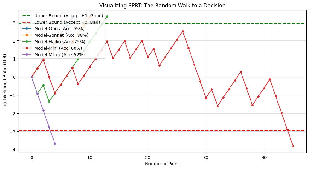
What this is showing us is that in this instance, the mini model took far longer than the rest to reach a concrete decision, this isn’t unexpected since it has a lower accuracy than the bigger models. Running this against all our models at scale reveals the following:
SPRT Parameters: p0=50.0%, p1=80.0%, alpha=0.05, beta=0.05
Log Bounds: Lower(A)=-2.944, Upper(B)=2.944

Model-Opus:
  Decision: Accept H1 (Accuracy is closer to 80.0%)
  Runs needed: 7 (vs ~thousands in CLT)
  True Accuracy: 95.0% | Sample Accuracy: 100.0%
  Estimated Cost: $0.175000

Model-Sonnet:
  Decision: Accept H1 (Accuracy is closer to 80.0%)
  Runs needed: 7 (vs ~thousands in CLT)
  True Accuracy: 88.0% | Sample Accuracy: 100.0%
  Estimated Cost: $0.052500

Model-Haiku:
  Decision: Accept H1 (Accuracy is closer to 80.0%)
  Runs needed: 16 (vs ~thousands in CLT)
  True Accuracy: 75.0% | Sample Accuracy: 81.2%
  Estimated Cost: $0.016000

Model-Mini:
  Decision: Accept H0 (Accuracy is closer to 50.0%)
  Runs needed: 14 (vs ~thousands in CLT)
  True Accuracy: 60.0% | Sample Accuracy: 50.0%
  Estimated Cost: $0.003500

Model-Micro:
  Decision: Accept H0 (Accuracy is closer to 50.0%)
  Runs needed: 10 (vs ~thousands in CLT)
  True Accuracy: 52.0% | Sample Accuracy: 40.0%
  Estimated Cost: $0.000500
As you can see we have dramatically cut the number of runs we need to get 95% confidence in our result, all the way from thousands in the previous step to between 5-20 depending on the model. We have also reduced the cost of these evaluations by orders of magnitude making it somewhat tractable to get a statistically significant result.
Considering Context
If we want to go further and squeeze even more juice out of a system like this, we can treat the problem like a router. This is sensible, since some models will be better at certain problems than others, and that won’t necessarily be captured in our aggregate accuracy, it will need to be learned. By using some basic features such as text embeddings and model ID you can begin to learn the accuracy of the model by predicting whether this collection of features will produce the finally decided result (this is a binary classification). A common architecture for this is a Gradient Boosted Tree.
Even though you are ultimately producing a binary result, you will have a confidence assigned to that binary result, in sklearn this is often the result of calling predict_proba. Unfortunately this is a poorly named function, as it doesn’t predict a probability, it actually just predicts confidence. To turn this confidence into a probability, we need to use calibration, a good method is Venn Abers, I would also recommend optimising the model against a stratified brier score so you end up with the best model for predicting a probability.
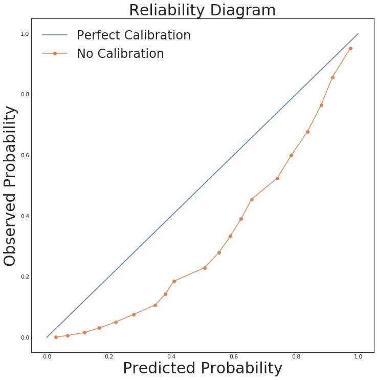
Now instead of using a global accuracy score, you can use an accuracy score for the model in the given context, and use that information in our SPRT system to come up with a confident assessment.
Covariance and the LLM Council
In our previous model, we assumed each model was independently predicting a result, and to certain extent that is true, its not like the models know what the others are predicting at any given moment, however these models are trained on data, and this training mechanism has biases that could ultimately lead models to produce similar results even if they don’t know what the other is predicting.
This means, our information gain should be somewhat related to how much these models agree with each other, if two models rarely agree with each other but agree on something, that is a signal of confidence. But how to model it?
Based on our training data, we know the accuracy of each model ID within a given context. We can then turn this into continuous uniformly distributed matrix by sampling figuring out the ground truth, then using randomised probability integral transform (RPIT). Now we have a matrix that isolates the “surprise” of our models, with bigger variances given to more discordant results.
Next we can use a Vine Copula to figure out our conditional probabilities. First we train a model, using a library like pyvinecopulib. Then lets say we are performing our SPRT run, we do the first run with no conditional probability. After this first run however, we have a result, and we can begin to assess the conditional information gain (and thus cost). Suppose on prompt X, we have model A with 80% accuracy, and model B with 80% accuracy, and lets say Kendalls rank correlation between these two models is very high (0.85). We ran A and observe that it failed (0 result), without the Vine Copula we would naively assume B has an 80% of being correct, but with our new system we can find a new updated conditional probability 22%, showing that B has almost no new information to give. We can take our GBT probabilities, put in our observed results (using RPIT), and find the conditional probabilities for all the remaining models for each loop.
These probabilities change our efficiency per token and we can simply select the one that gives us the best result each time, allowing us to lower our cost significantly. This allows you to do something like karpathys LLM council with statistical rigor.
How Confident is my Confidence?
Right now we are getting our probabilities from our GBT, and we are reasonably assured they are well calibrated, however there will always be times when something out of distribution comes up that we have to evaluate, such as a task we have never seen before. For this, we can use a technique known as Epistemic Uncertainty, where we look at the trees in our GBT and find out how much they disagree with each other (and how confidently).
To marry these values together (probability and uncertainty), we can use a beta distribution. Lets say we have probability P and epistemic variance U, we need to compute the maximum theoretical variance V of P (0.16):
Next we calculate our Method of Moments M (19):
Now we can extract our beta shape parameters:
This gives 15.2 for our alpha and 3.8 for our beta, meaning that the confidence our model has is equivalent to 15.2 positive and 3.8 negative outcomes.
We can use the M we calculated here to apply bayesian shrinkage around our GBT’s probability to get access to our informed probability I:
As M gets higher (indicating high confidence) our probability remains the same, as M gets smaller (indicating high uncertainty) our probability drifts further towards 0.5 (an uninformative prior).
With all this, we can be sure that our evals are providing reliable signals at the cheapest cost.